8. CP-predict: a two-phase algorithm for rRNA structure prediction

This page describes the secondary prediction algorithm developed specifically for rPredictorDB and ribosomal RNA.

Note

If you come across terminology or concepts you do not understand, you can try the rPredictorDB glossary or Biological background pages.

Note

CP-predict parameters are currently optimized for prokaryotic small subunit rRNA. A more general method of adapting parameters for each query separately is being developed.

8.1. Introduction

Ribosomal RNA molecules are a notoriously hard problem for RNA secondary structure prediction. They are long (at least 1500, some over 3500 nucleotides) and contain many unorthodox structural features: pseudoknots, non-canonical base pairs, modified residues, etc.

However, rRNA molecules exhibit a high level of homology - similarity across different taxa - both in sequences and higher-level structures, where structural homology is even stronger than sequence homology. When predicting the secondary structure of an rRNA molecule (further denoted as target), we can therefore use other rRNA with known structures as relatively good estimates of the target structure. A small but increasing number of rRNA structures has already been experimentally resolved, both for prokaryotic and eukaryotic organisms, which we can use as the structural templates as those target structure estimates.

Specifically, for each target molecule we choose a template molecule from a pre-determined set, align the target sequence to the template sequence and simply copy over the structure for corresponding positions. (This is why we refer to our algorithm also as “Cut-Paste prediction”, or CP-predict.)

However, while rRNA structure is conserved well in general, certain regions are not. Copying over the structure from these regions leads to worsened performance. To improve the prediction, we identify these unconserved regions and predict their secondary structure separately, using the Minimum Free Energy folding algorithm RNAfold of Hofacker et al. The unconserved regions typically have a length between 10 and 50 nucleotides, which is a scale at which minimum free energy folding works rather well.

Also, certain regions of the template structures have not been resolved (although the rest of the structure is). We also identify these unmeasured regions and use RNAfold to predict their structure. These regions range from 5 to over 100 nucleotides.

A third type of special regions are tangled regions. Because the ribosomal subunits often contain more than one rRNA molecule, some base pairs form between the different rRNAs. We identify regions of these base pairs and do not predict any base pairs for them; our prediction is concerned with single rRNA molecules only.

Taken together, the rPredict (or CP-predict) algorithm can be summarized as:

• Select a template,
• Align target to template,
• Identify unconserved and unmeasured regions,
• Copy template structure in conserved/measured regions to target,
• Predict structure for unconserved and unmeasured regions

8.2. Data

We need two kinds of data:

• template structures,
• a template profile alignment that we use to estimate conserved regions.

We use four template structures: one for the small ribosomal subunit and one for large ribosomal subunit of eukaryotic and prokaryotic organisms each. The template structures were extracted from PDB and secondary structure was obtained using the DSSR tool. We used templates with the following PDB IDs:

• 3J3F (H. Sapiens) for the eukaryotic large subunit,
• 3J3D (D. Melangoster) for the eukaryotic small subunit,
• 2AW4 (E. Coli) for the prokaryotic large subunit,
• 4JI1 (Th. Thermophilus) for the prokaryotic small subunit.

The template profiles were also obtained from PDB files with known structures, although in principle these could have been any rRNA sequences. We used molecules with resolved structures in order to be able to measure further properties and performance of rPredict (these will be gradually published on the site as experimentation progresses, hopefully culminating in a journal publication). We used the Clustalw2 tool to create the template profile alignments.

Note

CP-predict parameters are currently optimized for prokaryotic small subunit rRNA. A more general method of tuning parameters for each template separately is being developed.

In building the profile alignments, one also implicitly makes decisions about the balance of conserved and unconserved regions. If the profile is composed of sequences that are too similar, very few regions will be identified as unconserved, including those that are not conserved for a target molecule that further from the template. Therefore, the structure of these regions will be copied over to the target when it shouldn’t be. On the other hand, if the profile molecules are only loosely associated with each other, too many regions may be identified as unconserved and information from the template structure will be discarded unnecessarily (and RNAfold performation will deteriorate if the unconserved regions grow too long).

The proper amount of conservation depends on the other templates. Since we only use four templates, each for a very different category of rRNA, we can probably afford to have a bit more loosely associated molecules in template profiles, as long as they are molecules of the correct type (16S, 23S, etc.). Determining the proper amount of conservation (roughly expressed as the proportion of gaps in the resulting alignment, although one can use other measures, such as sum guide tree branch lengths) is an ongoing work.

8.3. rPredict algorithm

As has been said in the Introduction, the rPredict (or CP-predict) algorithm can be summarized as:

• Select a template,
• Align target to template,
• Identify unconserved and unmeasured regions,
• Copy template structure in conserved/measured regions to target,
• Predict structure for unconserved and unmeasured regions

We will now describe in detail the procedure for each step.

8.3.1. Template selection

We select the closest template simply by aligning the target sequence to all template sequences and choosing the tempate (one of the four mentioned in Data) closest to the target, as measured by distance in the guide tree. The alignment is computed by the clustalw2 command-line tool using default parameters.

8.3.2. Aligning target to template

We align the target sequence again, this time to the template profile alignment. Again, we use the clustalw2 command-line tool with default parameter values. (Experimentation with alignment parameters could lead to a significant improvement in prediction.) This alignment is referred to as target-template alignment, (tt-alignment) further in the text.

8.3.3. Conserved and unmeasured regions

We have discovered through experimentation that the regions in which copying template structure leads to poor prediction are generally those regions where more gaps appear in the tt-alignment. Therefore, we designed a sliding window algorithm, with parameters window_length and gap_threshold. The algorithm in pseudocode:

unconserved_regions = []

for each position in tt-alignment:
    current_window = tt-alignment[position:position + window_length]
    if proportion_of_gaps_in(current_window) > gap_threshold:
        if not in_unconserved_region:
            unconserved_region = (position, position + window_length)
            in_unconserved_region = True
        else:
            unconserved_region[1] = position + window_length
    else:
        if in_unconserved_region:
            unconserved_regions.append(unconserved_region)
        else:
            continue

return unconserved_regions

Furthermore, we do not count gaps that are at starts and end of sequences towards the gap threshold. This is because the alignment is rather unreliable at the sequence bounds; the alignment algorithm tends to favor gaps at ends over gaps in the middle and thus the level of conservation at sequence bounds is quite understated.

The parameters we found optimal by experimenting with a 7-sequence tt-alignment were a window of length 10 and the gap treshold set to 0.15. Decreasing the gap threshold without increasing window length leads to many very short unconserved regions; increasing window length without decreasing the gap threshold leads to a very strict algorithm that can miss significant unconserved regions. Ideally, we should be able to estimate optimal values for the parameters from the tt-alignment; this is reserved for future work.

Unmeasured regions of the template structure are mapped to the target using the target-tempate profile alignment.

8.3.4. Copying template to target structure

The template structure is simply copied over to the target, using the tt-alignment to map positions in the template to positions in the target. Base pairs that have one end mapped to a gap in the alignment are discarded (the other end is left unpaired). Also, only Watson-Crick and G-U Wobble pairs are retained.

Structure for unconserved regions is discarded (including base pairs that have one member outside the unconserved region; thanks to some unknown property of rRNAs, only very few such pairs exist, if the correct unconserved regions are identified). Structure for unmeasured and tangled regions is discarded as well. (However, for unmeasured regions, this does not make a difference, since all residues in the unmeasured regions of the template molecule are left unpaired in the template structure.)

8.3.5. Predicting structure for non-copied regions

We merge all unconserved and unmeasured regions (adjacent and overlapping regions are merged into one) and use RNAfold to predict the secondary structure of each of the merged non-copied region separately. Tangled regions are left unpaired.

8.4. Performance

To see how the algorithm works in practice, we will give you a step-by-step example. We will attempt to predict the structure of E. Coli 16S rRNA (entry 2AW7 in PDB, chain A), using the template structure of Thermus Thermophilus 16S rRNA (PDB ID 4JI1, chain A). We use secondary structure derived from the 2AW7 PDB file using DSSR as the reference structure against which performance is measured.

Note

The tool for visualizing structure comparisons draws seconary structures in a linear graph representation: nucleotides are arranged in a row and base pairs are indicated by arcs connecting the given nucleotides.

(The visualisation tool was kindly provided by Christina Witwer, author of the hxmatch algorithm.)

In the images:

• Red arcs represent base pairs that are in the predicted structure and should not be there (they are not present in the reference structure). The higher the percentage of red arcs, the worse the precision (also called specificity) of the prediction algorithm.
• Green arcs represent base pairs that are not predicted, but should be (they are in the reference structure). The higher the percentage of green arcs, the worse the recall (also called sensitivity).
• Black arcs represent correctly predicted base pairs. The more black base pairs, the better.

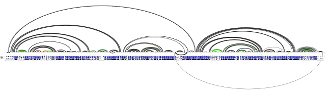
This is how the actual structures compare, after aligning 2AW7 to 4JI1 and collapsing the copied structure back to the unaligned form of 2AW7 (see Copying template to target structure, where we “freeze” the algorithm after removing base pairs that end in gaps and before we remove non-canonical base pairs):

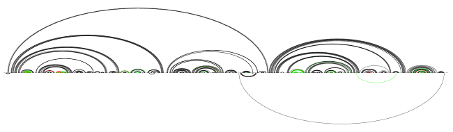
A simple copy of the target structure

The recall and precision stand at 85.1 and 91.0. This is a simple baseline. Notice the helices that are practically identical, only with one region shifted by a position or two: these make up most of the errors. This is the first one from the left:

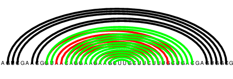
An example of a “shifted helix”

Also, notice that these helices do not have a large span; most helices spanning more than a few tens of nucleotides are predicted well by this rudimentary copy-paste. This is reinforces our belief that rRNA has nice conservation properties: the parts that are hard to guess from related structures are localized well.

Upon closer examination, we see that these one-off helices contain a large percentage of non-canonical base pairs. We therefore proceed to remove non-canonical base pairs:

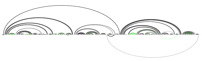
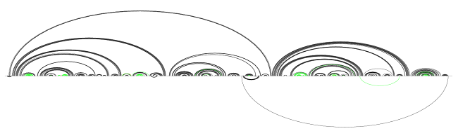
After non-canonical base pairs have been removed

Notice that the red/green helices have thinned. Removing base pairs never helps recall, but it helps precision (only red edges disappear). The trick is to remove only the base pairs that should not be in the structure. The non-canonical base pairs fit this bill nicely; the recall and precision stand at 85.1 and 96.2.

However, by sheer chance, some of the base pairs from the predicted shifted helices actually are canonical. The shifted helix from the previous example now looks like this:

Randomly canonical base pairs

If we tried to predict structures of the areas from which we just removed non-canonical base pairs, which are the likely suspect areas for non-conserved structure, we would find that these areas will be split into smaller pieces. If we ran structure prediction on them one by one, we wouldn’t be able to reconstruct the desired helices. If we ran the algorithm on all of them at once, we would get various erratic interactions between unrelated regions.

Therefore, we need a better heuristic to estimate where the unconserved regions lie. Simply looking for areas with non-canonical base pairs is a start, but not good enough.

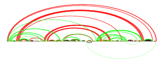
We noticed that the regions with problematic helices coincide with regions where gaps occur in the target-template profile alignment (the less blue and more white a region in the alignment, the more gaps and the less identity is in alignment in that region):

Problematic areas vs. alignment

Even more importantly, nearly all the green lines (i.e. base pairs missing from our prediction, which detracts from recall) occur in areas where conservation is sketchy at best, based at least on the simple identity check.

Note also that while the alignment bar is rather sparse at the ends of the structure, the structure is in fact conserved well in these regions. This is the observation that led us to exclude gaps at the starts and ends of template profile sequences from conservation tagging.

After running the sliding window conservation tagger, which looks for regions in the alignment where the percentage of gaps is larger than some threshold (see: Conserved and unmeasured regions), we obtained the following prediction:

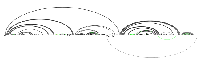
After removing base pairs from unconserved regions

Precision jumped considerably up again; out of the 380 predicted pairs, only 3 were incorrect. Recall, however, worsened slightly, as some base pairs were copied over correctly in areas tagged as unconserved. Recall and precision are now standing at 83.8 and 99.2.

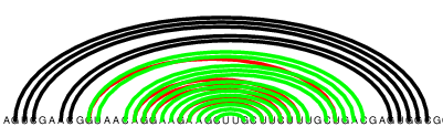
We now run RNAfold on the unconserved regions and obtain the following structure:

After predicting unconserved region structures

The performance is now at recall 88.0 and precision 97.6. Notice that we managed to improve recall, but hurt precision, albeit slightly: some extra base pairs were predicted and some base pairs missing before were actually predicted.

(Some experimentation was done on the parameters of the conservation tagger to find the optimal window size and gap threshold parameters. However, the optimal values of both depend on the specific alignment. A method for estimating the optima from the alignment is reserved for future work.)

8.4.1. Comparison vs. RNAfold

For a brief justification of CP-predict vs. using RNAfold for the entire structure: this is the prediction of RNAfold compared against the reference structure.

RNAfold prediction

8.4.2. Quantitative evaluation

We plan extensive performance tests, using all pairs of molecules in each template profile alignment as the template and target molecule. Also, to measure how well templates are selected and how much template selection matters, we will measure performance for an incorrectly chosen template. In the same vein, we can measure differences between corresponding prokaryotic and eukaryotic subunits.

Preliminary experimentation (predicting 16S rRNA from E. Coli and Th. Thermophilus without using RNAfold for non-copied regions) in the previous section suggest sensitivity/specificity 88.0/97.6, which is - to our knowledge - comparable with state-of-the-art models.