9. Structural features
Secondary structures are comprised of several types of elements, or “building blocks”. Each element can be characterised
We recognize the following structural features:
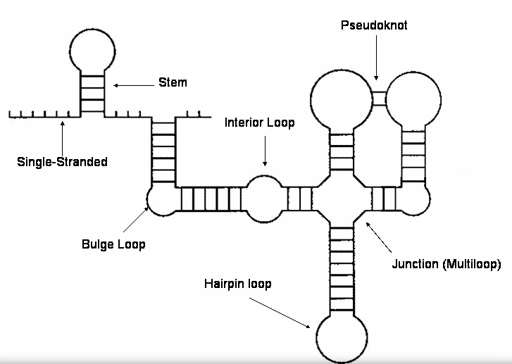
This is what these structural features look like on a typical secondary structure visualization:
(Image taken from http://kelder.zeus.ugent.be/~ide/open_dir/ website.)
9.1. Helix
A helix is a set of two regions (5’ side, 3’ side) of the same length such that all nucleotides are paired and that the i-th residue from start of the 5’ side is bound to the i-th residue from end of the 3’ side. In dot-paren representation, a helix looks like this:
((()))
The length of a helix is defined as the number of base pairs that participate in it. This is a deviation from the “clean” way, where the length of a structural feature is the number of positions participating in it; however, the base pair-based definition is the standard in literature.
Also known as: Stem
9.2. Hairpin loop
A hairpin loop is a region of unpaired residues flanked by a base pair. In dot-paren representation, a hairpin loop looks like this:
(......)
The length of a hairpin loop is the number of unpaired residues participating in it.
Also known as: Stem-loop
9.3. Internal loop
An internal loop is a pair of regions with the following dot-paren representation:
(...()....)
That is, the 3’-end of one region is paired to the 5’-end of the other and vice versa. All other residues are unpaired and there is at least one unpaired residue in both regions that make up the internal loop. The length of an internal loop is the number of unpaired residues participating in it.
9.4. Bulge
A bulge can be defined as a one-sided internal loop: one of the internal loop regions has no unpaired positions. In dot-paren representation:
(..())
The length of a bulge is the number of unpaired residues in the bulge. Again, this deviation from the norm is a literature standard.
9.5. Junction
A junction can also be derived from an internal loop: where an internal loop has two regions connected to each other by their 5’ and 3’-ends, a junction has multiple regions such that the i-th region’s 5’-end is connected to the i+1-th region’s 3’-end. In dot-paren representation:
(....()...()...)
The length of a junction is the number of participating residues, including the paired ones. The junction is k-fold if it includes k base pairs.
Junctions are called so because they represent a sub-structre from which multiple helices spawn in various directions, as opposed to an internal loop, which is just something like an intermission in a longer stem.
Also known as: Multi-loop, Multi-branch loop
9.6. 3’-overhang
The 3-overhang is the unpaired part (plus, for technical reasons, the first paired residue) at the 3’-end of the molecule. In dot-paren representation:
)....
The length of a 3-overhang is the number of unpaired residues participating in it.
9.7. 5’-overhang
The 5-overhang is the unpaired part (plus, for technical reasons, the first paired residue) at the 5’-end of the molecule. In dot-paren representation:
........(
The length of a 5-overhang is the number of unpaired residues participating in it.
9.8. Pseudoknot
A pseudoknot is a type of structure that breaks the well-nestedness of base pairs and helices. We define a pseudoknot as a set of helices that are in conflict. For instance, from the following dot-paren structure:
...(((..[[..)))..(((((..))(..)).))..((.(..]]..)))
we would have the following recorded as a pseudoknot:
((([[)))(((]])))
with the corresponding region designation. The length of a pseudoknot is the number of base pairs that break the well-nestedness (the square - or other - brackets in the dot-paren representation).
9.8.1. Assigning pseudoknottedness
The designation of which pairs are the pseudoknotted ones and which are the well-nested ones is a non-trivial task. From the following options:
...((.[[))...]]..
...[[.((]]...))..
which one should we choose? The rPredictorDB pseudoknot algorithm is based on vertex coloring of the helix conflict graph, a data structure in which helices represent vertices and edges lead between helices that are in conflict (that are not well-nested w.r.t. each other). Our “colors” are levels of pseudoknotted-ness, denoted by different bracket styles: ‘(‘ is a non-pseudoknot, ‘[‘ is a level-1 pseudoknot, ‘{‘ is a level-2 pseudoknot, etc. We then use a greedy BFS coloring algorithm:
- To the current vertex, we try to assign the highest-possible priority color. Highest priority is ‘(‘, then ‘[‘, etc. - in effect, we are trying to greedily minimize the amount of pseudoknotted helices (not necessarily base pairs).
- The first vertex to be colored from each connected component of the conflict graph is the one with the highest degree (most conflicts).
- Neighbors are added to the coloring BFS queue ordered from highest to lowest degree.
- The starting color is ‘[‘ if the starting vertex degree is at least 1. Trivial components (just one vertex - conflict-free helices) are colored ‘(‘. This is a heuristic that tries to minimize the number of pseudoknot helices: if we take as the pseudoknot helix the one with most conflicts, we are maximizing the number of helices that may then be without further conflicts.
9.8.2. Pseudoknot types
Pseudoknots are classified into further types (currently not recognized by rPredictorDB, but a possible avenue of extension):
H-type loops:
...((((..[.[[.))).)..]]]
“Kissing hairpins”:
...((.[[))..(((.]].)))..
Three-knot:
...((.[[..{)).]].}...
The three-knots can get more complicated, of course: ..((.[[{.)).((.])).]..}, etc. Higher-level knots, while theoretically possible, are not widely known in RNA.
