1. rWeb Tutorial

Note

The website is known to work for the major browsers in their current version: Mozilla Firefox, Internet Explorer (10+) and Google Chrome.

The website offers two functionalities: search and prediction of secondary structure. Since both are only loosely related, we’ll give a separate tutorial for each. Only the “Search” and “Predict” pages offer site functionalities, so the tutorial will focus exclusively on them.

The most important part of the documentation is The rPredictorDB Toolkit and the The rPredictorDB Toolkit Reference. The first document, The rPredictorDB Toolkit, will help you select which tools are appropriate for the job you want to do. The second document, The rPredictorDB Toolkit Reference, will tell you exactly how to use the selected tool. Make sure you read the introductory remarks for both the Search tools and Prediction tool after the tutorial!

The next most important part is the rPredictorDB glossary, which should make terminology clear.

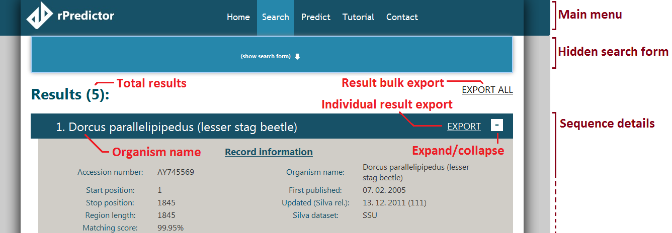
First of all, however, we need to agree on what various parts of the site layout are called. The following picture should clarify how we call layout elements:

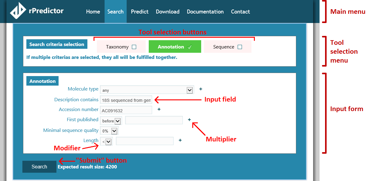
Search page layout

The Predict page is practically identical.

1.1. Search tutorial

Let’s say our lab colleague brought some strange beetles he discovered the other day in his back yard. We want to know whether they are a new species and how they should be classified phylogenetically. So, we obtain the ribosomal RNAs and head to rPredictorDB.

First, we can check whether the sequence already exists in the database. This is an exact search task and, according to The rPredictorDB Toolkit, the appropriate tool for the job is the Sequence search. In The rPredictorDB Toolkit Reference, we find out that there is a search field directly for matching the exact (sub)sequence. So, we head to the Search page.

1.1.1. Using the Search form

On the Search page, we find out that the Database search tool is selected by default, so we don’t have to select it and the Database search form is available right away. We will copy-paste our sequence into the Sequence input field.

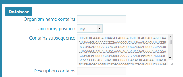
Sequence input into Database search tool

We will select no other criteria for now and click “Search”.

Note

Next to the submit button, an estimate of how many database entries match your search is given. This number is no more than an estimate; when and how it is computed and updated is still under construction.

Search button & estimated number of results

When searching, the search form will roll up and hide (there is a “Show search form” button to roll it back down). The search screen will look like this:

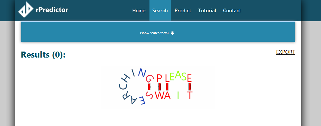
Waiting screen

Searching for an exact sequence/subsequence takes a bit longer, because we have to check against a lot of starting positions in the half-million sequences we have in the database. However, soon enough, we find out that there is no match for our sequence (the “Searching please wait” animation stops).

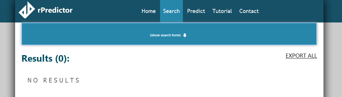
Search finished, no results found

Our beetle’s rRNA sequence was not found in the database; so far it looks like we found a new species!

But then we realize that maybe we made some error in the sequencing process, or there could be a mutation in our specimen, or the database has a mutated specimen - in any case, maybe an exact search was not the best way to confirm that our beetle is a new guy to the party. So we check the The rPredictorDB Toolkit for tools that may be better suited for the task. It so turns out that there are similarity search tools, BLAST and BLAT, that can show us all rRNA sequences similar to our beetle’s rRNA. If a sequence differs in only very few positions, or only at the 3’ or 5’ end, there’s a good chance that our beetle is, in the end, not from a new species.

Based on the description in the toolkit overview, we chose BLAST for the search, so that we are sure not to miss any potentially similar sequence.

1.1.2. Selecting tools

We head back to the search form (for instance by clicking “Show search form”) and look at the tool selection menu. Again, by default, the “Database” tool is selected.

Tool selection menu

The selection menu reflects the current search form status - if you want to select a tool, click the red button, if you want to unselect a tool, click the green button. In our case, we want to cancel Database search and use BLAST alone, so we click the Database button (so that it now has the red “X” next to it) and the BLAST button (so that it now has a green tick). Notice how the search forms for the tools disappear and appear on click. The tool selection menu will now look like this:

Tool selection menu, after switching Database search for BLAST

Each tool selection button contains in the alt-text a (very) brief description of the tool.

We now copy & paste our sequence to the Sequence input field of the BLAST tool search form. Last, we need to decide on the minimum level of similarity we want to report (checking against The rPredictorDB Toolkit Reference). Given our scenario, we settle on 98 % similarity and click Search.

1.1.3. Reading search results

Lo and behold, there are results! Maybe our beetle is not such a find. We are met with the result screen. The layout is described in the following figure:

Result screen

When searching yields results, they are displayed as sequence details. The first sequence detail is displayed in the fully expanded version, the others are displayed in their short versions. The fully expanded sequence detail is rather long. Use the ‘-‘ sign in the upper right corner of the first detail to collapse the first detail (and see the others).

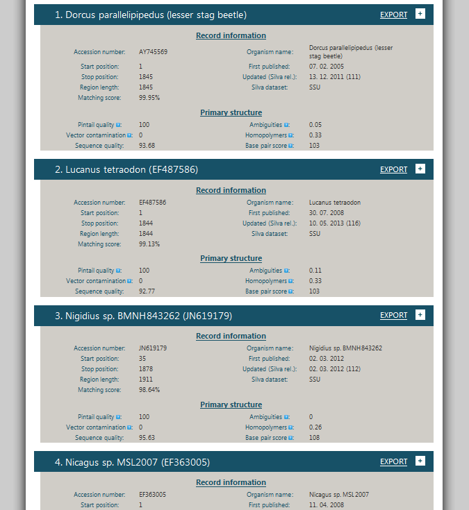
There are more results than just the first one!

Only the first twenty results are displayed for browsing at first. If you want to browse more, scroll to the bottom and click the and the following twenty will be retrieved (and so on, and so forth).

1.1.4. Sequence detail

The sequence detail is at a first glance a rather intimidating beast. Let us take it apart, step by step. (For a full description of each detail field, see rPredictorDB record detail.)

The (expanded) sequence detail consists of multiple sections (taken from Overview of available information):

• General information: basic information about the database record: accession number, organism name, datataset, etc. A full description is here: General information.
• Primary structure: information about the primary structure - start position, stop position, sequence quality, etc. A full description is here: Primary structure.
• Secondary structure: fields pertaining to the predicted secondary structure of the sequence - the predicted structure in dot-paren notation, a summary of structural features and a visualization of the structure. The tool which was used for predicting the secondary structure is also given. The visualization is just a thumbnail; if you click it, the full-size image will be generated on the fly in a new tab/window. A full description is here: Secondary structure.
• References: references to scientific literature pertinent to the rPredictorDB record. A full description is here: References.
• Features: various other fields defined in the data sources. This section cannot be relied upon to be present everywhere in the same form. A full description is here: Specimen.
• Xrefs: cross-references to other data sources from which the rPredictorDB record was assembled. A full description is here: Xrefs.

Each section has a heading (in bold blue text) and a set of fields. The section headings for References, Features and Xrefs are clickable and show/hide the given section on click.

1.1.5. Exporting

You can also export the search results in various format.

On the result screen (Result screen), notice the “Individual export button” on the right of the detail header. If we click it, the following screen comes up:

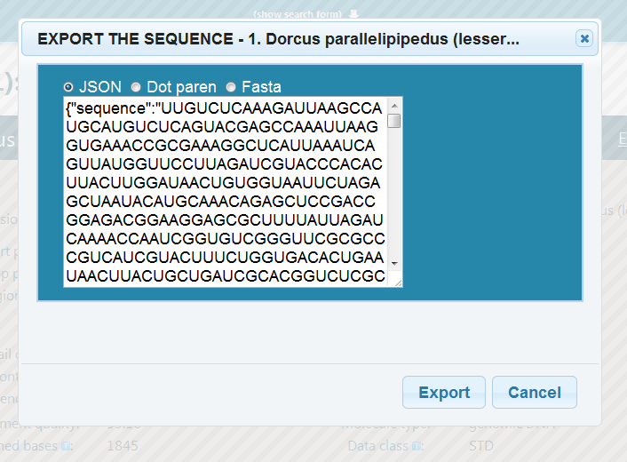
Export screen

There is a selection of export formats above the text area in the middle. The text area is a preview for the exported file. Clicking “Export” starts the download of an export.json (or .html, or other suffixes for other formats) file with the contents given in the text area.

To exit the export dialogue and go back to browsing results, either click Cancel on the bottom, or the X in the upper right corner.

You can also mass-export all results, or a subset, by clicking on the Export all button. The following dialogue will appear:

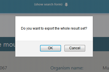
Dialogue on exporting the entire result set

If you select Yes, the export screen will appear; this time with the preview of the list of all retrieved records. Its behavior is identical to the single-sequence export case.

If you select No, you will see that the Export all button changed: instead of just Export all, there is a choice:

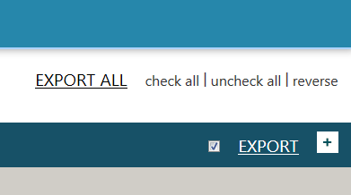
Options for mass export

and a checkbox appears to the left of the individual export button. “Export all” from now on means “Export all checked”. Check all and Uncheck all are self-explanatory, Reverse simply reverses the selection.

Because the retrieved records are loaded on demand in sets of 5, if you want the mass export right away, you’ll have to wait until the remaining records are retrieved from the database. The following screen will come up:

Waiting for export results

1.2. Prediction tutorial

Secondary structure prediction is even easier than search, both on the input side and on the output. The use of the prediction form and tool selection is exactly the same as for search: see Using the Search form and Selecting tools, with one important distinction: only one prediction tool can be selected at the same time. (This also means we don’t have to de-select tools, simply click the prediction tool you want to use and the previous tool will de-select automatically.)

Currently, all prediction input forms even are the same: they require a FASTA header (complete with the > sign as the first character) and a sequence. The header can be omitted; if it is, the result will show a no header text.

1.2.1. Prediction output

The prediction results look like this:

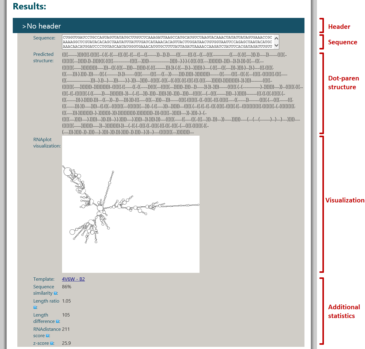
Prediction results

The visualization is generated by RNAplot, which ignores the predicted pseudoknots.

1.3. Analyse tutorial

rPredictorDB infrastructure contains analytical module that can do different tasks with the data you have found using Search tutorial.

First thing you need to do is search and store some sequences. You already know how to search the sequences, so what you need to do now, is search something - you can try putting “Homo sapiens” in the organism name field for instance. In the results of the search, you pick some sequences that you want to use for analysing later. You simply check the checboxes in the header of each record next to expand/collapse icon. When you’re done selecting sequences, scroll back to the top of the page and click “Save for analysis” button. You’ll be notified that sequences has been stored and now you can simply go to Analyse modul (via main menu).

In the Analyse module, you have three main columns - first is displaying your stored datasets. Dataset is basically list of sequences that you have selected in the previous step (in the Search). Datasets are named by date they were created. Once you stored multiple datasets, you can choose between them by clicking them in this list.

Second column displays sequences belonging to selected dataset. Here you can select, which subset of the stored dataset will be used for analysis. Finally, in the third column is a list of tools that you can use for the analysis. Simply click the button here and you’ll see the results depending on tool chosen.